Chapitre 10 La mise en page de plusieurs graphiques

Le package cowplot permet la combinaison de plusieurs graphiques. Il est composé de plusieurs fonctions.

• la fonction plot_grid qui permet de disposer n graphes sur i colonnes et j lignes

gg1 <- ggplot(ODD_graphique1) +
  geom_point(aes(
    x = Gross_Domestic_Product_GDP,
    y = Maternal_mortality_ratio
  )) +
  scale_x_log10() +
  scale_y_log10() +
  labs(
    title = "Mortalité maternelle en fonction du PIB par habitant",
    subtitle = "En 2015",
    x = "PIB",
    y = "Taux de mortalité de la mère \n(pour 100 000 naissances)",
    caption = "Source : ODD / ONU"
  ) +
  theme(axis.title = element_text(size = 9))

gg2 <- ggplot(ODD_graphique1) +
  geom_density(aes(x = log(Gross_Domestic_Product_GDP)))

plot_grid(gg1, gg2, ncol = 1, nrow = 2)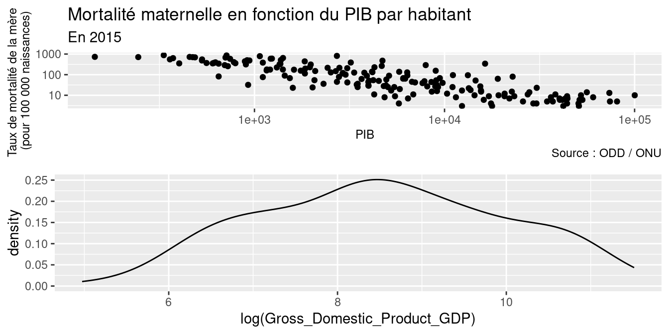

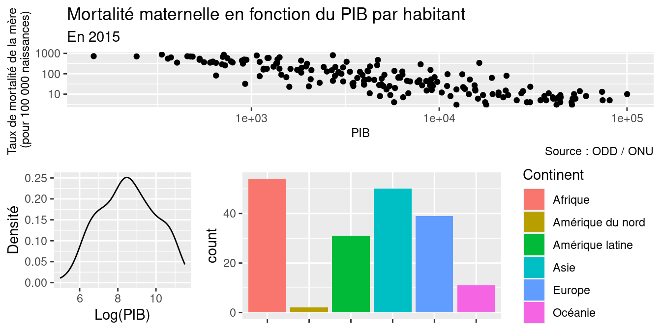
• la fonction draw_plot associée à ggdraw qui permet de disposer les graphiques à des places spécifiques

ggdraw initialise le graphique

gg1 <- ggplot(ODD_graphique1) +
  geom_point(aes(x = Gross_Domestic_Product_GDP,
    y = Maternal_mortality_ratio)) +
  scale_x_log10() +
  scale_y_log10() +
  labs(title = "Mortalité maternelle en fonction du PIB par habitant",
    subtitle = "En 2015",
    x = "PIB",
    y = "Taux de mortalité de la mère \n(pour 100 000 naissances)",
    caption = "Source : ODD / ONU") +
  theme(axis.title = element_text(size = 9))

gg2 <- ggplot(ODD_graphique1) +
  geom_density(aes(x = log(Gross_Domestic_Product_GDP))) +
  labs(x = "Log(PIB)",
    y = "Densité")

gg3 <- ggplot(data = ODD_graphique1) +
  geom_bar(aes(x = Continent, fill = Continent)) +
  theme(axis.title.x = element_blank(),
    axis.text.x = element_blank())

ggdraw() +
  draw_plot(gg1, x = 0, y = .5, width = 1, height = .5) +
  draw_plot(gg2, x = 0, y = 0, width = .3, height = .5) +
  draw_plot(gg3, x = 0.3, y = 0, width = 0.7, height = .5)