Tutoriel didor
tutoriel_didor.RmdDIDO
- Un catalogue à disposition du public, utilisable avec {didor}
- Un système d’alimentation du catalogue pour les agents qui alimentent régulièrement DIDO
Catalogue
On trouve ici le catalogue DIDO : https://www.statistiques.developpement-durable.gouv.fr/catalogue?page=explore&type=dataset&pagination=1&sortField=last_modified&sortOrder=desc
Des jeux de données et des fichiers de données
DIDO propose aujourd’hui (23/02/2023) Une vingtaine de jeux de données (dataset) et environ 120 fichiers de données (datafile).
1 ou plusieurs fichiers de données sont inclus dans un jeu de données. Chaque jeu de données contient des fichiers d’annexes.
La logique est donc la suivante : on explore DIDO en commençant par chercher le dataset qui nous intéresse, puis on trouve la donnée en explorant les datafiles avec l’aide des annexes. Ces annexes commentent et précisent la nature des informations contenues dans les datafiles qui constituent un ensemble logique d’informations : le dataset exploré.
Que l’on peut aussi explorer directement avec R {didor}
{didor} est un package R https://github.com/MTES-MCT/didor
qui propose une documentation de prise en main :
https://mtes-mct.github.io/didor/articles/premiers_pas.html
Explorons
Il va nous falloir des fonctions du tidyverse
## ── Attaching core tidyverse packages ──────────────────────── tidyverse 2.0.0 ──
## ✔ dplyr     1.1.1     ✔ readr     2.1.4
## ✔ forcats   1.0.0     ✔ stringr   1.5.0
## ✔ ggplot2   3.4.1     ✔ tibble    3.2.1
## ✔ lubridate 1.9.2     ✔ tidyr     1.3.0
## ✔ purrr     1.0.1
## ── Conflicts ────────────────────────────────────────── tidyverse_conflicts() ──
## ✖ dplyr::filter() masks stats::filter()
## ✖ dplyr::lag()    masks stats::lag()
## ℹ Use the conflicted package (<http://conflicted.r-lib.org/>) to force all conflicts to become errors
je voudrais la liste des jeux de données proposés
tbl_dataset <- didor::datasets()| title | spatial_granularity |
|---|---|
| Données locales de consommation d’électricité et de gaz naturel et de chaleur et de froid - adresse (à partir de 2018) | poi |
| Données locales de consommation d’électricité et de gaz naturel - région (à partir de 2018) | fr:region |
| Conjoncture mensuelle de l’énergie | country |
| Données nationales sur la commercialisation des logements neufs | country |
| Données régionales sur la commercialisation des logements neufs | fr:region |
je voudrais la liste des fichiers de données proposés
Disons que je m’interesse à ce jeu de donnée :
Indicateurs territoriaux de développement durable (ITDD)
J’ai envie d’écrire cela :
| title | description |
|---|---|
| Données de consommation et de points de livraison d’énergie à la maille adresse - électricité - année 2018 | Consommations d’électricité et points de livraison, par secteur d’activité (agriculture, industrie, tertiaire, résidentiel et non affecté), à la maille géographique adresse |
| Données de consommation et de points de livraison d’énergie à la maille adresse - électricité - année 2019 | Consommations d’électricité et points de livraison, par secteur d’activité (agriculture, industrie, tertiaire, résidentiel et non affecté), à la maille géographique adresse |
| Données de consommation et de points de livraison d’énergie à la maille adresse - électricité - année 2020 | Consommations annuelles et nombre de points de livraison d’électricité des bâtiments professionnels par secteur d’activité (agriculture, industrie, tertiaire et non affecté) et de ceux du secteur résidentiel d’au moins 10 logements à la maille adresse |
| Données de consommation et de points de livraison d’énergie à la maille adresse - électricité - année 2021 | Consommations annuelles et nombre de points de livraison d’électricité des bâtiments professionnels par secteur d’activité (agriculture, industrie, tertiaire, résidentiel et non affecté) ou selon le code NAF à 2 niveaux selon les cas et de ceux du secteur résidentiel d’au moins 10 logements à la maille adresse |
| Données de consommation et de points de livraison d’énergie à la maille adresse - gaz naturel - année 2018 | Consommations annuelles et nombre de points de livraison de gaz naturel des bâtiments professionnels par secteur d’activité (agriculture, industrie, tertiaire et non affecté) et de ceux du secteur résidentiel d’au moins 10 logements ou de plus de 200 MWh à la maille adresse |
Trop de résultats au milieu de tous les fichiers de données ! Les infos des fichiers de données ne permettent pas de filtrer sur les jeux de données auxquels ils appartiennent.
Il faut donc d’abord sélectionner le jeu de données qui nous intéresse :
brutalement par exemple :
tbl_dataset <- didor::datasets() %>%
dplyr::filter(title %in% c("Indicateurs territoriaux de développement durable (ITDD)"))| title | spatial_granularity |
|---|---|
| Indicateurs territoriaux de développement durable (ITDD) | fr:commune |
ou avec la fonction dido_search :
tbl_dataset <- didor::datasets() %>%
didor::dido_search("ITDD")| title | spatial_granularity |
|---|---|
| Indicateurs territoriaux de développement durable (ITDD) | fr:commune |
Peu importe le moyen, on peut maintenant chercher les fichiers contenus dans le jeu de données :
tbl_datafile_itdd <- didor::datasets() %>%
  didor::dido_search("ITDD") %>%
didor::datafiles()| title | description |
|---|---|
| 1.01 ITDD - France entière | Les données des indicateurs territoriaux correspondant aux 17 objectifs de développement durable. Couverture : France entière Granularité : nationale |
| 1.02 ITDD - France hors Mayotte | Les données des indicateurs territoriaux correspondant aux 17 objectifs de développement durable. Couverture : France hors Mayotte Granularité : nationale |
| 1.03 ITDD - France métropolitaine | Les données des indicateurs territoriaux correspondant aux 17 objectifs de développement durable. Couverture : France métropolitaine Granularité : nationale |
| 2.01 ITDD - Province de France métropolitaine | Les données des indicateurs territoriaux correspondant aux 17 objectifs de développement durable. Couverture : Province de France métropolitaine Granularité : province |
| 3.01 ITDD - Toutes régions | Les données des indicateurs territoriaux correspondant aux 17 objectifs de développement durable. Couverture : France entière Granularité : régions Code Officiel Géographique INSEE (N-1 du millésime) |
Même ainsi, il y a du choix !
je voudrais un fichier de données dans un dataframe
Donc on en sélectionne un :
tbl_datafile_itdd <- didor::datasets() %>%
  didor::dido_search("ITDD") %>%
  didor::datafiles() %>%
didor::dido_search("Bourgogne-Franche-Comté")| title | description |
|---|---|
| 5.08 ITDD - Bourgogne-Franche-Comté - Toutes les communes | Les données des indicateurs territoriaux correspondant aux 17 objectifs de développement durable. Couverture : région Bourgogne-Franche-Comté Granularité : communes Code Officiel Géographique INSEE (N-1 du millésime) |
Et on le récupère : on le met dans un tibble.
C’est quoi un tibble ?
https://tibble.tidyverse.org/
Il est donc chargé en mémoire dans R.
tbl_datafile_itdd <- didor::datasets() %>%
  didor::dido_search("ITDD") %>%
  didor::datafiles() %>%
  didor::dido_search("Bourgogne-Franche-Comté") %>%
  didor::get_data(query = c(
    columns = "CODGEO_CODE,CODGEO_LIBELLE,A2019,A2018,A2017",
    # NO_INDIC ="eq:i021",
    VARIABLE = "eq:ESO_PES_NB_TOT_CLAS4",
    NO_INDIC ="eq:i034b"
  ))
## ℹ downloading data and caching to : /tmp/Rtmppimz9y/eb8b9bd5-8e50-4007-a869-948781aadeb3-2023-01-columns=CODGEO_CODE,CODGEO_LIBELLE,A2019,A2018,A2017;VARIABLE=eqESO_PES_NB_TOT_CLAS4;NO_INDIC=eqi034b.csv##
Downloading: 10 B
Downloading: 10 B
Downloading: 7 kB
Downloading: 7 kB
Downloading: 8.2 kB
Downloading: 8.2 kB
Downloading: 8.2 kB
Downloading: 8.2 kB
Downloading: 10 kB
Downloading: 10 kB
Downloading: 12 kB
Downloading: 12 kB
Downloading: 12 kB
Downloading: 12 kB
Downloading: 12 kB
Downloading: 12 kB
Downloading: 16 kB
Downloading: 16 kB
Downloading: 16 kB
Downloading: 16 kB
Downloading: 16 kB
Downloading: 16 kB
Downloading: 20 kB
Downloading: 20 kB
Downloading: 25 kB
Downloading: 25 kB
Downloading: 25 kB
Downloading: 25 kB
Downloading: 25 kB
Downloading: 25 kB
Downloading: 28 kB
Downloading: 28 kB
Downloading: 28 kB
Downloading: 28 kB
Downloading: 28 kB
Downloading: 28 kB
Downloading: 30 kB
Downloading: 30 kB
Downloading: 31 kB
Downloading: 31 kB
Downloading: 31 kB
Downloading: 31 kB| CODGEO_CODE | CODGEO_LIBELLE | A2019 | A2018 | A2017 |
|---|---|---|---|---|
| 21001 | Agencourt | 0 | 0 | 0 |
| 21002 | Agey | 0 | 0 | 0 |
| 21003 | Ahuy | 0 | 0 | 0 |
| 21004 | Aignay-le-Duc | 0 | 0 | 0 |
| 21005 | Aiserey | 0 | 0 | 0 |
| 21006 | Aisey-sur-Seine | 0 | 0 | 0 |
| 21007 | Aisy-sous-Thil | 0 | 0 | 0 |
| 21008 | Alise-Sainte-Reine | 0 | 0 | 0 |
| 21009 | Allerey | 0 | 0 | 0 |
| 21010 | Aloxe-Corton | 0 | 0 | 0 |
| 21011 | Ampilly-les-Bordes | 0 | 0 | 0 |
| 21012 | Ampilly-le-Sec | 0 | 0 | 0 |
| 21013 | Ancey | 0 | 0 | 0 |
| 21014 | Antheuil | 0 | 0 | 0 |
| 21015 | Antigny-la-Ville | 0 | 0 | 0 |
| 21016 | Arceau | 0 | 0 | 0 |
| 21017 | Arcenant | 0 | 0 | 0 |
| 21018 | Arcey | 0 | 0 | 0 |
| 21020 | Arconcey | 0 | 0 | 0 |
| 21021 | Arc-sur-Tille | 0 | 0 | 0 |
| 21022 | Argilly | 0 | 0 | 0 |
| 21023 | Arnay-le-Duc | 0 | 0 | 0 |
| 21024 | Arnay-sous-Vitteaux | 0 | 0 | 0 |
| 21025 | Arrans | 0 | 0 | 0 |
| 21026 | Asnières-en-Montagne | 0 | 0 | 0 |
| 21027 | Asnières-lès-Dijon | 0 | 0 | 0 |
| 21028 | Athée | 0 | 0 | 0 |
| 21029 | Athie | 0 | 0 | 0 |
| 21030 | Aubaine | 0 | 0 | 0 |
| 21031 | Aubigny-en-Plaine | 0 | 0 | 0 |
Mais qu’est ce que c’est que ces paramètres dans get_data ?
{didor} ne fait rien d’autre que proposer les mêmes outils que ceux dont on dispose dans le catalogue :
- selectionner des colonnes
- filtrer les lignes selon un critère sur une variable ou plusieurs
paramètres
didor::get_data() peut prendre un paramètre query et ce n’est qu’une requête écrite et passée à l’API.
On trouve donc des informations qui permettent de s’y retrouver dans la documentation de l’API du fichier de données :
Les annexes
Dans l’onglets métadonnées du fichier de données ou après les
fichiers de données, dans le jeu de données.
On peut les consulter en ligne ou directement les récupérer via
didor::attachments()
  tbl_attachment <- didor::datasets() %>%
    didor::dido_search("ITDD") %>%
    didor::attachments() %>%
    didor::dido_search("6.01") %>%
    didor::get_attachments(dest = tempdir())
## file downloaded: /tmp/Rtmppimz9y/dictionnaire-indicateurs-territoriaux-developpement-durable.xlsxtypage
Les données sont toutes en chr : pour les manipuler ce n’est pas forcément pratique. C’est néanmoins nécessaire, pourquoi ?
Dans un datafile, une variable (colonne) numérique contient une valeur qui peut être manquante. Le producteur de la donnée peut, s’il le souhaite, préciser la raison de l’absence. “secret” indiquera que la valeur sous secret statistique
Donc dans DIDO, (numérique) est équivalent à (type numérique de R union “secret”) Bref, en utilisant la fonction convert(), on supprime tout cela et on peut effectuer des opérations mathématiques.
str(tbl_datafile_itdd)## tibble [3,700 × 5] (S3: tbl_df/tbl/data.frame)
## $ CODGEO_CODE : chr [1:3700] "21001" "21002" "21003" "21004" ...
## ..- attr(*, "name")= chr "CODGEO_CODE"
## ..- attr(*, "description")= chr "COG_COMMUNE - Code de la zone"
## ..- attr(*, "unit")= chr "n/a"
## ..- attr(*, "type")= chr "string"
## ..- attr(*, "converted")= logi FALSE
## $ CODGEO_LIBELLE: chr [1:3700] "Agencourt" "Agey" "Ahuy" "Aignay-le-Duc" ...
## ..- attr(*, "name")= chr "CODGEO_LIBELLE"
## ..- attr(*, "description")= chr "COG_COMMUNE - Libellé de la zone"
## ..- attr(*, "unit")= chr "n/a"
## ..- attr(*, "type")= chr "string"
## ..- attr(*, "converted")= logi FALSE
## $ A2019 : chr [1:3700] "0" "0" "0" "0" ...
## ..- attr(*, "name")= chr "A2019"
## ..- attr(*, "description")= chr "A2019"
## ..- attr(*, "unit")= chr "n/a"
## ..- attr(*, "type")= chr "number"
## ..- attr(*, "converted")= logi FALSE
## $ A2018 : chr [1:3700] "0" "0" "0" "0" ...
## ..- attr(*, "name")= chr "A2018"
## ..- attr(*, "description")= chr "A2018"
## ..- attr(*, "unit")= chr "n/a"
## ..- attr(*, "type")= chr "number"
## ..- attr(*, "converted")= logi FALSE
## $ A2017 : chr [1:3700] "0" "0" "0" "0" ...
## ..- attr(*, "name")= chr "A2017"
## ..- attr(*, "description")= chr "A2017"
## ..- attr(*, "unit")= chr "n/a"
## ..- attr(*, "type")= chr "number"
## ..- attr(*, "converted")= logi FALSEIl suffit de les convertir avec la fonction convert()
tbl_datafile_itdd <- didor::datasets() %>%
  didor::dido_search("ITDD") %>%
  didor::datafiles() %>%
  didor::dido_search("Bourgogne-Franche-Comté") %>%
  didor::get_data(query = c(
    columns = "CODGEO_CODE,CODGEO_LIBELLE,A2019,A2018,A2017",
    # NO_INDIC ="eq:i021",
    VARIABLE = "eq:ESO_PES_NB_TOT_CLAS4",
    NO_INDIC ="eq:i034b"
  )) %>%
  didor::convert()
## ℹ reading data from cache : /tmp/Rtmppimz9y/eb8b9bd5-8e50-4007-a869-948781aadeb3-2023-01-columns=CODGEO_CODE,CODGEO_LIBELLE,A2019,A2018,A2017;VARIABLE=eqESO_PES_NB_TOT_CLAS4;NO_INDIC=eqi034b.csv
str(tbl_datafile_itdd) ## tibble [3,700 × 5] (S3: tbl_df/tbl/data.frame)
## $ CODGEO_CODE : chr [1:3700] "21001" "21002" "21003" "21004" ...
## ..- attr(*, "name")= chr "CODGEO_CODE"
## ..- attr(*, "description")= chr "COG_COMMUNE - Code de la zone"
## ..- attr(*, "unit")= chr "n/a"
## ..- attr(*, "type")= chr "string"
## ..- attr(*, "converted")= logi FALSE
## $ CODGEO_LIBELLE: chr [1:3700] "Agencourt" "Agey" "Ahuy" "Aignay-le-Duc" ...
## ..- attr(*, "name")= chr "CODGEO_LIBELLE"
## ..- attr(*, "description")= chr "COG_COMMUNE - Libellé de la zone"
## ..- attr(*, "unit")= chr "n/a"
## ..- attr(*, "type")= chr "string"
## ..- attr(*, "converted")= logi FALSE
## $ A2019 : num [1:3700] 0 0 0 0 0 0 0 0 0 0 ...
## ..- attr(*, "name")= chr "A2019"
## ..- attr(*, "description")= chr "A2019"
## ..- attr(*, "unit")= chr "n/a"
## ..- attr(*, "type")= chr "number"
## ..- attr(*, "converted")= logi TRUE
## $ A2018 : num [1:3700] 0 0 0 0 0 0 0 0 0 0 ...
## ..- attr(*, "name")= chr "A2018"
## ..- attr(*, "description")= chr "A2018"
## ..- attr(*, "unit")= chr "n/a"
## ..- attr(*, "type")= chr "number"
## ..- attr(*, "converted")= logi TRUE
## $ A2017 : num [1:3700] 0 0 0 0 0 0 0 0 0 0 ...
## ..- attr(*, "name")= chr "A2017"
## ..- attr(*, "description")= chr "A2017"
## ..- attr(*, "unit")= chr "n/a"
## ..- attr(*, "type")= chr "number"
## ..- attr(*, "converted")= logi TRUECherchons une correlation
Par exemple, entre la participation au présidentielles 2022 et le taux de 20/24 ans sortis non diplomés
result <- didor::datasets() %>%
  didor::dido_search("ITDD") %>%
  didor::datafiles() %>%
  didor::dido_search("Bourgogne-Franche-Comté") %>%
  didor::get_data(query = c(
    columns = "VARIABLE,CODGEO_CODE,CODGEO_LIBELLE,A2022,A2019,A2017,A2013,A2012,A2007,A2002",
    # NO_INDIC ="eq:i021",
    # VARIABLE = "eq:taux_participation"
    VARIABLE = "in:part_20_24_sortis_nondip,taux_participation"
    #NO_INDIC ="eq:i110"
  )) %>%
  didor::convert() %>%
  dplyr::select(CODGEO_CODE,A2022,A2019) %>%
  group_by(CODGEO_CODE) %>%
  summarise_at(c("A2022","A2019"),sum,na.rm=T)
## ℹ downloading data and caching to : /tmp/Rtmppimz9y/eb8b9bd5-8e50-4007-a869-948781aadeb3-2023-01-columns=VARIABLE,CODGEO_CODE,CODGEO_LIBELLE,A2022,A2019,A2017,A2013,A2012,A2007,A2002;VARIABLE=inpart_20_24_sortis_nondip,taux_participation.csv##
Downloading: 10 B
Downloading: 10 B
Downloading: 7 kB
Downloading: 7 kB
Downloading: 8.2 kB
Downloading: 8.2 kB
Downloading: 8.2 kB
Downloading: 8.2 kB
Downloading: 8.2 kB
Downloading: 8.2 kB
Downloading: 12 kB
Downloading: 12 kB
Downloading: 12 kB
Downloading: 12 kB
Downloading: 12 kB
Downloading: 12 kB
Downloading: 16 kB
Downloading: 16 kB
Downloading: 16 kB
Downloading: 16 kB
Downloading: 16 kB
Downloading: 16 kB
Downloading: 20 kB
Downloading: 20 kB
Downloading: 25 kB
Downloading: 25 kB
Downloading: 25 kB
Downloading: 25 kB
Downloading: 25 kB
Downloading: 25 kB
Downloading: 27 kB
Downloading: 27 kB
Downloading: 28 kB
Downloading: 28 kB
Downloading: 28 kB
Downloading: 28 kB
Downloading: 28 kB
Downloading: 28 kB
Downloading: 33 kB
Downloading: 33 kB
Downloading: 33 kB
Downloading: 33 kB
Downloading: 33 kB
Downloading: 33 kB
Downloading: 36 kB
Downloading: 36 kB
Downloading: 37 kB
Downloading: 37 kB
Downloading: 37 kB
Downloading: 37 kB
Downloading: 37 kB
Downloading: 37 kB
Downloading: 37 kB
Downloading: 37 kB
Downloading: 45 kB
Downloading: 45 kB
Downloading: 45 kB
Downloading: 45 kB
Downloading: 45 kB
Downloading: 45 kB
Downloading: 45 kB
Downloading: 45 kB
Downloading: 53 kB
Downloading: 53 kB
Downloading: 53 kB
Downloading: 53 kB
Downloading: 53 kB
Downloading: 53 kB
Downloading: 53 kB
Downloading: 53 kB
Downloading: 57 kB
Downloading: 57 kB
Downloading: 57 kB
Downloading: 57 kB
Downloading: 57 kB
Downloading: 57 kB
Downloading: 60 kB
Downloading: 60 kB
Downloading: 60 kB
Downloading: 60 kB
Downloading: 60 kB
Downloading: 60 kB
Downloading: 68 kB
Downloading: 68 kB
Downloading: 68 kB
Downloading: 68 kB
Downloading: 68 kB
Downloading: 68 kB
Downloading: 68 kB
Downloading: 68 kB
Downloading: 72 kB
Downloading: 72 kB
Downloading: 72 kB
Downloading: 72 kB
Downloading: 72 kB
Downloading: 72 kB
Downloading: 72 kB
Downloading: 72 kB
Downloading: 72 kB
Downloading: 72 kB
Downloading: 80 kB
Downloading: 80 kB
Downloading: 80 kB
Downloading: 80 kB
Downloading: 80 kB
Downloading: 80 kB
Downloading: 82 kB
Downloading: 82 kB
Downloading: 84 kB
Downloading: 84 kB
Downloading: 85 kB
Downloading: 85 kB
Downloading: 85 kB
Downloading: 85 kB
Downloading: 85 kB
Downloading: 85 kB
Downloading: 88 kB
Downloading: 88 kB
Downloading: 88 kB
Downloading: 88 kB
Downloading: 88 kB
Downloading: 88 kB
Downloading: 88 kB
Downloading: 88 kB
Downloading: 96 kB
Downloading: 96 kB
Downloading: 96 kB
Downloading: 96 kB
Downloading: 96 kB
Downloading: 96 kB
Downloading: 96 kB
Downloading: 96 kB
Downloading: 100 kB
Downloading: 100 kB
Downloading: 100 kB
Downloading: 100 kB
Downloading: 100 kB
Downloading: 100 kB
Downloading: 110 kB
Downloading: 110 kB
Downloading: 110 kB
Downloading: 110 kB
Downloading: 110 kB
Downloading: 110 kB
Downloading: 110 kB
Downloading: 110 kB
Downloading: 110 kB
Downloading: 110 kB
Downloading: 110 kB
Downloading: 110 kB
Downloading: 110 kB
Downloading: 110 kB
Downloading: 120 kB
Downloading: 120 kB
Downloading: 120 kB
Downloading: 120 kB
Downloading: 120 kB
Downloading: 120 kB
Downloading: 120 kB
Downloading: 120 kB
Downloading: 130 kB
Downloading: 130 kB
Downloading: 130 kB
Downloading: 130 kB
Downloading: 130 kB
Downloading: 130 kB
Downloading: 130 kB
Downloading: 130 kB| CODGEO_CODE | A2022 | A2019 |
|---|---|---|
| 21001 | 77.71 | 33.65 |
| 21002 | 80.74 | 33.33 |
| 21003 | 81.13 | 16.95 |
| 21004 | 74.58 | 23.08 |
| 21005 | 81.55 | 8.20 |
En en faisant un nuage de points :
ggplot(result, aes(x=A2022, y=A2019)) + geom_point()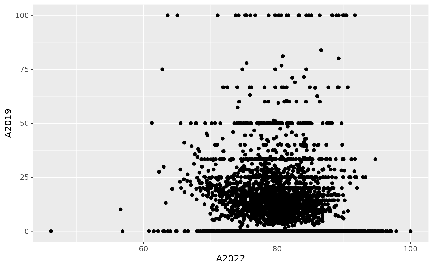
eco-considérations
Les données sont récupérées, et transitent donc sur le réseau
lorsqu’on fait un get_data() et les paramètres de la
‘query’ du get_data() filtrent et sélectionnent les données
qui sont transférées.
Le filtrage/sélection s’effectue dans DiDo.
Si on avait tout récupéré sans filtrer/sélectionner on aurait envoyé environ 20 millions de lignes et un bon paquet de colonnes au travers du réseau, ça aurait pris du temps… probablement planté… et consommé plein de ressources inutiles…
Bref, filtrer/sélectionner au plus près de DIDO, c’est mieux !
On peut faire du {shiny} avec {didor}
On peut utiliser {didor} dans une appli {shiny} un exemple avec les données NAMEA d’emission de GES
library(shiny)
library(didor)
library(stringr)

code_nace <-   datasets() %>%
  dido_search('NAMEA') %>%
  datafiles() %>%
  get_data(
    query = c(columns = "CODE_NACE_REV2_ET_MENAGES,LIBELLE_NACE_ET_MENAGES")
  )
shinyApp(

# Define UI for application that draws a histogram
ui <- fillPage(
  tags$style(HTML('
    body {
        font-family: "Helvetica Neue",Helvetica,Arial,sans-serif;
        font-size: 7px;
        line-height: 1.42857143;
        color: #333;
        background-color: #fff;
    }
    ')),
    # Application title
    titlePanel("{didor}+{shiny}"),

    # Sidebar with a slider input for number of bins
    sidebarLayout(
      sidebarPanel(
        selectInput(
          inputId = "nace",
          label = "code nace",
          choices = unique(code_nace$LIBELLE_NACE_ET_MENAGES)
        ),
        width=2
      ),
      mainPanel(
        tableOutput("table"),
        width=10
      )
    )
),

# Define server logic required to draw a histogram
server <- function(input, output) {

  code_nace_select <- reactive({
    str_c(
      "in:",
      as.character(
        dplyr::filter(
          unique(
            code_nace
          ),
          LIBELLE_NACE_ET_MENAGES %in% c(input$nace))[1])
    )

  })

  data <- reactive({
    datasets() %>%
      dido_search('NAMEA') %>%
      datafiles() %>%
      get_data(
        query = c(SUBSTANCE="in:GES",CODE_NACE_REV2_ET_MENAGES=code_nace_select())
      )
  })
  output$table <- renderTable(data())
},

options = list(width = "100%",height = 500)

)
# Run the application
shinyApp(ui = ui, server = server)
Crédits
Merci à Nicolas Chuche pour la construction de {didor} et merci à vous de vos retours sur son utilisation : nous vous invitons à ouvrir des issues dans github afin de nous permettre d’améliorer ce package : https://github.com/MTES-MCT/didor/issues
(et merci à Olivier Chantrel pour ce tutoriel !)